import pandas as pd
import numpy as np
import matplotlib.pyplot as plt
import tensorflow as tf

import random
import warnings
warnings.filterwarnings("ignore")

import nibabel as nib
import cv2
from PIL import Image
from shutil import copyfile, copyfileobj
import PIL

from sklearn.model_selection import train_test_split
from sklearn.utils import class_weight
from sklearn.metrics import roc_auc_score


from tensorflow.keras.callbacks import Callback
from tensorflow.keras import datasets, layers, models
from tensorflow.keras.losses import binary_crossentropy
from tensorflow.keras.models import Model, load_model, Sequential
from tensorflow.keras.layers import Input, BatchNormalization, Activation, Dense, Dropout, Flatten
from tensorflow.keras.layers import  Conv2D, Conv2DTranspose, MaxPooling2D, GlobalMaxPooling2D
from tensorflow.keras.layers import concatenate, Add
from tensorflow.keras.layers import Lambda, RepeatVector, Reshape
from tensorflow.keras.callbacks import EarlyStopping, ModelCheckpoint, ReduceLROnPlateau, LearningRateScheduler
from tensorflow.keras.optimizers import Adam
from tensorflow.keras.preprocessing.image import ImageDataGenerator, array_to_img, img_to_array, load_img
from tensorflow.keras import backend as K
from pylab import rcParams
# Read and examine metadata
raw_data = pd.read_csv('/content/covid19-ct-scans/metadata.csv')
raw_data = raw_data.replace('../input/covid19-ct-scans/','/content/covid19-ct-scans/',regex=True)
print(raw_data.shape)
raw_data.head(5)
Preprocessing Images
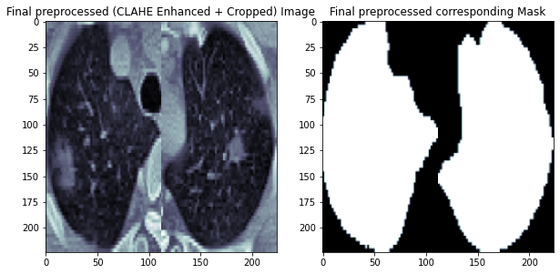
The preprocessing steps are the same as we did in Part I, including CLAHE enhancement and crop the lung regions in the CT scans.
CLAHE Enhance
Used (CLAHE) Contrast Limited Adaptive Histogram Equalization to enhance the contrast of the images since medical images suffer a lot from the contrast problems.
Cropping
Each CT scan in our dataset has its corresponding lungs mask. We can use the lungs mask to find out the ROI for cropping. So we can image for a possible complete Covid-19 diagonsis pipeline can be:
- First, semantic segmentation to get the lungs mask.
- Second, using the lungs mask to crop the ROIs.
- Then, send the ROIs to a classifier for Covid-19 diagnosis.
def clahe_enhancer(img, demo=False):
    img = np.uint8(img*255)
    clahe = cv2.createCLAHE(clipLimit=3.0, tileGridSize=(8,8))
    clahe_img = clahe.apply(img)
    if demo:
        img_flattened = img.flatten()
        clahe_img_flattened = clahe_img.flatten()
        fig = plt.figure()
        rcParams['figure.figsize'] = 10,10

        plt.subplot(2, 2, 1)
        plt.imshow(img, cmap='bone')
        plt.title("Original CT-Scan")

        plt.subplot(2, 2, 2)
        plt.hist(img_flattened)
        plt.title("Histogram of Original CT-Scan")

        plt.subplot(2, 2, 3)
        plt.imshow(clahe_img, cmap='bone')
        plt.title("CLAHE Enhanced CT-Scan")

        plt.subplot(2, 2, 4)
        plt.hist(clahe_img_flattened)
        plt.title("Histogram of CLAHE Enhanced CT-Scan")

    return clahe_img

def cropper(test_img, demo):

    test_img = test_img*255
    test_img = np.uint8(test_img)
    contours,hierarchy = cv2.findContours(test_img, cv2.RETR_TREE, cv2.CHAIN_APPROX_SIMPLE)
    areas = [cv2.contourArea(c) for c in contours]

    x = np.argsort(areas)
    max_index = x[x.size - 1]
    cnt1=contours[max_index]
    second_max_index = x[x.size - 2]
    cnt2 = contours[second_max_index]
    x,y,w,h = cv2.boundingRect(cnt1)
    p,q,r,s = cv2.boundingRect(cnt2)
    cropped1 = test_img[y:y+h, x:x+w]
    cropped1 = cv2.resize(cropped1, dsize=(125,250), interpolation=cv2.INTER_AREA)
    cropped2 = test_img[q:q+s, p:p+r]
    cropped2 = cv2.resize(cropped2, dsize=(125,250), interpolation=cv2.INTER_AREA)

    if x < p:
        fused = np.concatenate((cropped1, cropped2), axis=1)
    else:
        fused = np.concatenate((cropped2, cropped1), axis=1)

    points_lung1 = []
    points_lung2 = []
    points_lung1.append(x); points_lung1.append(y); points_lung1.append(w); points_lung1.append(h)
    points_lung2.append(p); points_lung2.append(q); points_lung2.append(r); points_lung2.append(s)

    if demo == 1:
        fig = plt.figure()
        rcParams['figure.figsize'] = 35, 35
        plt.subplot(1, 3, 1)
        plt.imshow(test_img, cmap='bone')
        plt.title("Original CT-Scan")
        plt.subplot(1, 3, 2)
        plt.imshow(thresh, cmap='bone')
        plt.title("Binary Mask")
        plt.subplot(1, 3, 3)
        plt.imshow(fused, cmap='bone')
        plt.title("Cropped CT scan after making bounding rectangle")
        # plt.subplot(1, 4, 4)
        # plt.imshow(super_cropped, cmap='bone')
        # plt.title("Cropped further manually")
        plt.show()
    return (fused, points_lung1, points_lung2)
Following is an example CT scan after preprocessing and its corresponding lung mask image.
Load and Prepare Data
Define a function to read .nii files
The dataset contains CT scans with masks of 20 cases of Covid-19. There are 20 .nii files in each folder of the dataset. Each .nii file contains around 180 slices (images). Total slices are 3520. These have been sliced out by 20% in the front and by 20% in the last of each file since in general these didn't had any infection masks and some didn't had the lungs, removed as noise. Also, images had pixel values in a very large range. We need to normalize the pixel values.
def read_nii(filepath, data):
    '''
    Reads .nii file and returns pixel array
    '''
    ct_scan = nib.load(filepath)
    array   = ct_scan.get_fdata()
    array   = np.rot90(np.array(array))
    slices = array.shape[2]
    array = array[:,:,round(slices*0.2):round(slices*0.8)]
    array = np.reshape(np.rollaxis(array, 2),(array.shape[2],array.shape[0],array.shape[1], 1))

    for img_no in range(0, array.shape[0]):
        # array = Image.resize(array[...,img_no], (img_size,img_size))
        img = cv2.resize(array[img_no], dsize=(img_size, img_size), interpolation=cv2.INTER_AREA)
        xmax, xmin = img.max(), img.min()
        img = (img - xmin)/(xmax - xmin)
        data.append(img)
cts = []
lungs = []
img_size = 224
for i in range(0, 20):
    read_nii(raw_data.loc[i,'lung_mask'], lungs)
    read_nii(raw_data.loc[i,'ct_scan'], cts)

len(cts), len(lungs)
Drop NaN Data
Some masks in the dataset contain only nan values, so we need to drop both these masks and their corresponding CT scans
nan_list = []
for img_id in range(len(lungs)):
    if np.isnan(lungs[img_id].sum()):
        nan_list.append(img_id)
print(nan_list)

del lungs[1368:1372]
del cts[1368:1372]
del lungs[1924:1926]
del cts[1924:1926]
Perform Data Preprocessing
CLAHE enhancement and cropping.
new_lungs = []
new_cts = []

for img_id in range(len(lungs)):
    lung_img = lungs[img_id]
    lung_img[lung_img>0] = 1
    cropped_lung, points1, points2 = cropper(lung_img, demo=0)
    cropped_lung = cv2.resize(cropped_lung, (224, 224))
    new_lungs.append(cropped_lung)
    # print(len(points1), len(points2))

    cts_img = cts[img_id]
    cts_img = clahe_enhancer(cts_img, demo=False)

    a,b,c,d = points1[0], points1[1], points1[2], points1[3]
    e,f,g,h = points2[0], points2[1], points2[2], points2[3]
    img1 = cts_img[b:b+d, a:a+c]
    img1 = cv2.resize(img1, dsize=(125,250), interpolation=cv2.INTER_AREA)
    img2 = cts_img[f:f+h, e:e+g]
    img2 = cv2.resize(img2, dsize=(125,250), interpolation=cv2.INTER_AREA)
    if a<e:
        cropped_cts = np.concatenate((img1, img2), axis=1)
    else:
        cropped_cts = np.concatenate((img2, img1), axis=1)
    cropped_cts = cv2.resize(cropped_cts, (224, 224))
    new_cts.append(cropped_cts)

print(len(new_cts), len(new_lungs))
new_cts = np.uint8(np.array(new_cts))
new_lungs = np.uint8(np.array(new_lungs))
new_cts = new_cts/255
new_lungs = new_lungs/255
Below we plot a few examples of the processed CT scans and their corresponding masks.
def plot_sample(array_list, color_map = 'jet'):
    '''
    Plots and a slice with all available annotations
    '''
    fig = plt.figure(figsize=(10,30))

    plt.subplot(1,2,1)
    plt.imshow(array_list[0].reshape(224, 224), cmap='bone')
    plt.title('Original Image')

    plt.subplot(1,2,2)
    plt.imshow(array_list[0].reshape(224, 224), cmap='bone')
    plt.imshow(array_list[1].reshape(224, 224), alpha=0.5, cmap=color_map)
    plt.title('Lungs Mask')
    plt.show()

for index in [100,110,120,130,140,150]:
    plot_sample([new_cts[index], new_lungs[index]])


Data Augmentation
Since we only have 2106 training images and masks, it is a good practice to increase the size of our dataset by performing some data augmentation. To make it simple, I only add the left-right flip and up-down flip of the original images and original masks.
You code use the code below to do data augmentation, but it is not a necessary step.
aug_cts = []
aug_lungs = []

def augmentation(imgs, masks):
    for i in range(imgs.shape[0]):
        img = imgs[i,:,:]
        mask = masks[i, :, :]
        aug_cts.append(img)
        aug_lungs.append(mask)

        img_lr = np.fliplr(img)
        mask_lr =np.fliplr(mask)
        img_ud = np.flipud(img)
        mask_ud = np.flipud(mask)
        aug_cts.append(img_lr)
        aug_lungs.append(mask_lr)
        aug_cts.append(img_ud)
        aug_lungs.append(mask_ud)

augmentation(new_cts, new_lungs)
new_cts = np.array(aug_cts)
new_lungs = np.array(aug_lungs)
Following shows a few examples of augemented results.
for index in [100,110,120,130,140,150]:
    plot_sample([new_cts[index], new_lungs[index]])


# define building blocks
def BatchActivate(x):
    x = BatchNormalization()(x)
    x = Activation('relu')(x)
    return x

def convolution_block(x, filters, size, strides=(1,1), padding="same", activation=True):
    x = Conv2D(filters, size, strides=strides, padding=padding)(x)
    if activation == True:
        x = BatchActivate(x)
    return x

def residual_block(blockInput, num_filters=16, batch_activate=False):
    x = BatchActivate(blockInput)
    x = convolution_block(x, num_filters, (3,3))
    x = convolution_block(x, num_filters, (3,3), activation=False)
    x = Add()([x, blockInput])
    if batch_activate:
        x = BatchActivate(x)
    return x
def build_model(input_layer, start_neurons, DropoutRatio = 0.5):

    conv1 = Conv2D(start_neurons * 1, (3, 3), activation=None, padding="same")(input_layer)
    conv1 = residual_block(conv1,start_neurons * 1)
    conv1 = residual_block(conv1,start_neurons * 1, True)
    pool1 = MaxPooling2D((2, 2))(conv1)
    pool1 = Dropout(DropoutRatio/2)(pool1)

    conv2 = Conv2D(start_neurons * 2, (3, 3), activation=None, padding="same")(pool1)
    conv2 = residual_block(conv2,start_neurons * 2)
    conv2 = residual_block(conv2,start_neurons * 2, True)
    pool2 = MaxPooling2D((2, 2))(conv2)
    pool2 = Dropout(DropoutRatio)(pool2)

    conv3 = Conv2D(start_neurons * 4, (3, 3), activation=None, padding="same")(pool2)
    conv3 = residual_block(conv3,start_neurons * 4)
    conv3 = residual_block(conv3,start_neurons * 4, True)
    pool3 = MaxPooling2D((2, 2))(conv3)
    pool3 = Dropout(DropoutRatio)(pool3)

    conv4 = Conv2D(start_neurons * 8, (3, 3), activation=None, padding="same")(pool3)
    conv4 = residual_block(conv4,start_neurons * 8)
    conv4 = residual_block(conv4,start_neurons * 8, True)
    pool4 = MaxPooling2D((2, 2))(conv4)
    pool4 = Dropout(DropoutRatio)(pool4)

    convm = Conv2D(start_neurons * 16, (3, 3), activation=None, padding="same")(pool4)
    convm = residual_block(convm,start_neurons * 16)
    convm = residual_block(convm,start_neurons * 16, True)

    deconv4 = Conv2DTranspose(start_neurons * 8, (3, 3), strides=(2, 2), padding="same")(convm)
    uconv4 = concatenate([deconv4, conv4])
    uconv4 = Dropout(DropoutRatio)(uconv4)

    uconv4 = Conv2D(start_neurons * 8, (3, 3), activation=None, padding="same")(uconv4)
    uconv4 = residual_block(uconv4,start_neurons * 8)
    uconv4 = residual_block(uconv4,start_neurons * 8, True)

    deconv3 = Conv2DTranspose(start_neurons * 4, (3, 3), strides=(2, 2), padding="same")(uconv4)
    uconv3 = concatenate([deconv3, conv3])
    uconv3 = Dropout(DropoutRatio)(uconv3)

    uconv3 = Conv2D(start_neurons * 4, (3, 3), activation=None, padding="same")(uconv3)
    uconv3 = residual_block(uconv3,start_neurons * 4)
    uconv3 = residual_block(uconv3,start_neurons * 4, True)

    deconv2 = Conv2DTranspose(start_neurons * 2, (3, 3), strides=(2, 2), padding="same")(uconv3)
    uconv2 = concatenate([deconv2, conv2])

    uconv2 = Conv2D(start_neurons * 2, (3, 3), activation=None, padding="same")(uconv2)
    uconv2 = residual_block(uconv2,start_neurons * 2)
    uconv2 = residual_block(uconv2,start_neurons * 2, True)

    deconv1 = Conv2DTranspose(start_neurons * 1, (3, 3), strides=(2, 2), padding="same")(uconv2)
    uconv1 = concatenate([deconv1, conv1])

    uconv1 = Conv2D(start_neurons * 1, (3, 3), activation=None, padding="same")(uconv1)
    uconv1 = residual_block(uconv1,start_neurons * 1)
    uconv1 = residual_block(uconv1,start_neurons * 1, True)

    output_layer = Conv2D(1, (1,1), padding="same", activation="sigmoid")(uconv1)

    return output_layer
Define Metrics
We first define metrics for training our model. We use the dice coefficient and dice loss. Dice coeffient is the ratio between 2 * intersection (of true mask and predicted mask) and the sum of true and predicted masks. I refered to this site.
def dice_coef(y_true, y_pred):
    smooth = 1.
    y_true_f = K.flatten(y_true)
    y_pred_f = K.flatten(y_pred)
    intersection = K.sum(y_true_f * y_pred_f)
    score = (2. * intersection + smooth) / (K.sum(y_true_f) + K.sum(y_pred_f) + smooth)
    return score

def dice_loss(y_true, y_pred):
    loss = 1 - dice_coef(y_true, y_pred)
    return loss
Data generator to load data to our model
def Generator(X_list, y_list, batch_size = 32):
    c = 0
    while True:

        X = X_list[c:c+batch_size, :,:]
        y = y_list[c:c+batch_size, :, :]

        X = X[:,:,:,np.newaxis]
        y = y[:,:,:,np.newaxis]

        c += batch_size
        if (c+batch_size >= len(X_list)):
            c = 0
        yield X, y
Training Model
We first split the augmented dataset into training and validation sets (0.8:0.2).
We train the model for 80 epochs with a batch_size of 16. We set a ModelCheckpoint to save the model with the best val_dice_coef.
x_train, x_valid, y_train, y_valid = train_test_split(
    new_cts, new_lungs, test_size=0.2, random_state=42)

epochs = 80
batch_size = 16
steps_per_epoch = int(len(x_train) / batch_size)
validation_steps = int(len(x_valid) / batch_size)

train_gen = Generator(x_train, y_train, batch_size = batch_size)
val_gen = Generator(x_valid, y_valid, batch_size = batch_size)
# initialize our model
inputs = Input((img_size, img_size, 1))
output_layer = build_model(inputs, 16, 0.5)
# Define callbacks to save model with best val_dice_coef
checkpointer = ModelCheckpoint(filepath = 'best_lungs_224_res.h5', monitor='val_dice_coef', verbose=1, save_best_only=True, mode='max')
model = Model(inputs=[inputs], outputs=[output_layer])
model.compile(optimizer=Adam(lr = 3e-5), loss=dice_loss, metrics=[dice_coef])
results = model.fit(train_gen, steps_per_epoch=steps_per_epoch, epochs = epochs,
                             validation_data = val_gen, validation_steps = validation_steps,callbacks=[checkpointer])
After training 80 epochs, we obtain a model with a best val_dice_coef of 0.97673, which is very close to 1. We can expect our model will perform well.
Epoch 79/80
105/105 [==============================] - ETA: 0s - loss: 0.0217 - dice_coef: 0.9783
Epoch 00079: val_dice_coef improved from 0.97539 to 0.97622, saving model to best_lungs_224_res.h5
105/105 [==============================] - 35s 334ms/step - loss: 0.0217 - dice_coef: 0.9783 - val_loss: 0.0238 - val_dice_coef: 0.9762
Epoch 80/80
105/105 [==============================] - ETA: 0s - loss: 0.0214 - dice_coef: 0.9786
Epoch 00080: val_dice_coef improved from 0.97622 to 0.97673, saving model to best_lungs_224_res.h5
105/105 [==============================] - 35s 334ms/step - loss: 0.0214 - dice_coef: 0.9786 - val_loss: 0.0233 - val_dice_coef: 0.9767
Model Evaluation
We evaluate the model performance by looking at the training and validation dice coefficient of the training process.
As we can see from the figure below, the training and validation dice_coef have a very similar trend. No over-fitting or under-fitting can be observed.
!cp drive/My\ Drive/Colab\ Notebooks/models/best_lungs_res_224_model.h5 ./
model.load_weights("best_lungs_res_224_model.h5")
fig, loss_ax = plt.subplots()

acc_ax = loss_ax.twinx()

loss_ax.plot(results.history['loss'], 'y', label='train loss')
loss_ax.plot(results.history['val_loss'], 'r', label='val loss')

acc_ax.plot(results.history['dice_coef'], 'b', label='train dice coef')
acc_ax.plot(results.history['val_dice_coef'], 'g', label='val dice coef')

loss_ax.set_xlabel('epoch')
loss_ax.set_ylabel('dice loss')
acc_ax.set_ylabel('dice coefficient')

loss_ax.legend(loc='upper left')
acc_ax.legend(loc='lower left')

plt.show()

The score on validation set is ~0.9773.
score = model.evaluate(x_valid, y_valid, batch_size=32)
print("test loss, test dice coefficient:", score)
Visualize the results
We compare a few examples of true masks and our predicted masks by randomly selecting 5 images from our validation set.
As we can see from the below images, our predicted masks are very close to the true masks. They have a good cover on the lungs regions in the CT scans.
def compare_true_and_predicted(image_id):
    temp = model.predict(x_valid[image_id].reshape(1,img_size, img_size, 1))

    fig = plt.figure(figsize=(15,15))

    plt.subplot(1,3,1)
    plt.imshow(x_valid[image_id].reshape(img_size, img_size), cmap='bone')
    plt.axis("off")
    plt.title('Original Image (CT)')

    plt.subplot(1,3,2)
    plt.imshow(y_valid[image_id].reshape(img_size,img_size), cmap='bone')
    plt.axis("off")
    plt.title('True mask')

    plt.subplot(1,3,3)
    plt.imshow(temp.reshape(img_size,img_size), cmap='bone')
    plt.axis("off")
    plt.title('Predicted mask')

    plt.show()
rand = np.random.randint(0, len(x_valid), size=5)
for i in rand:
    compare_true_and_predicted(i)


Summary
In this post, we've built a U-Net with Residual blocks to predict lungs masks in CT scans. U-Net in general, has a good performance on medical images. It is good for semantic segmentation, although it can do instance segmentation as well.
Our trained model have a very good performance on predicting the lungs masks. The trained model will be used in a whole automatic Covid-19 diagnosis pipeline. Stay tuned for Part III of the Covid-19 series.
Comments
comments powered by Disqus