Foetal Head Segmentation on Ultrasound Images using Residual U-Net¶

Measuring foetal head circumference is one of the most accurate method to estimate gestational age after the first trimester (first three months of pregnancy). To automate this procedure, the most important step is segment the foetal head area in ultrasound images. Then we can fit an ellipse on the head area, and build a regressor using the head mask to estimate gestational age.

In this post, we will use a U-Net architecture with residual blocks to make head segmentations. U-Net performs very well on medical images. And due to its relatively compact structure, its speed is much faster than Mask-RCNN.

U-Net Structure¶

The U-Net architecture is shown below.

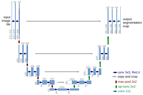
The provided model is basically a convolutional auto-encoder, but with a twist - it has skip connections from encoder layers to decoder layers that are on the same "level". In this post, we will use residual blocks to replace the simple convolutional blocks to increase the complexity of the model.

Note: the number of filters we use is different from the above picture. Find details in the model building section.

We are using a custom dataset with around 1000 training images and training masks, and 300 test ultrasound images.

In [1]:

# import necessary libraries
import os
import re
import numpy as np
import pandas as pd
import matplotlib.pyplot as plt

import cv2
from PIL import Image
from skimage.transform import resize
from sklearn.model_selection import train_test_split

import tensorflow.keras
import tensorflow as tf
from tensorflow.keras import backend as K

K.set_image_data_format('channels_last')

Understanding the Dataset¶

The foetal head ultrasound image dataset has two directories, train and test. The train folder contains the 999 training images and their corresponding masks. The test folder contains 335 test images. The sturcture are as follows:

foetal-head-us/
    train/
        000_HC.png
        000_HC_Mask.png
        001_HC.png
        001_HC_Mask.png
        ...
    test/
        000_HC.png
        001_HC.png
        ...

The training masks are named as training image name + '_Mask.png"

Load the Data¶

Set File Path

In [2]:

# training data path
path_train = "foetal-head-us/train/"
file_list_train = sorted(os.listdir(path_train))

#test data path
path_test = "foetal-head-us/test/"
file_list_test = sorted(os.listdir(path_test))

Separate Training Images and Masks

In [3]:

train_image = []
train_mask = []
for idx, item in enumerate(file_list_train):
    if idx % 2 == 0:
        train_image.append(item)
    else:
        train_mask.append(item)
print("Number of US training images is {}".format(len(train_image)))
print("Number of US training masks is {}".format(len(train_mask)))  
print(train_image[:5],"\n" ,train_mask[:5])

Number of US training images is 999
Number of US training masks is 999
['000_HC.png', '001_HC.png', '002_HC.png', '003_HC.png', '004_HC.png'] 
 ['000_HC_Mask.png', '001_HC_Mask.png', '002_HC_Mask.png', '003_HC_Mask.png', '004_HC_Mask.png']

Visualize an Example of Training Data

Following is an example from the training data. The image on the left is the ultrasound image, the image in the middle is its mask, image on the right shows an overlapping of the training mask and training image.

In [4]:

# Display the first image and mask of the first subject.
image1 = np.array(Image.open(path_train+"009_HC.png"))
image1_mask = np.array(Image.open(path_train+"009_HC_Mask.png"))
# binary inverse the mask
image1_mask = np.ma.masked_where(image1_mask == 0, image1_mask)

fig, ax = plt.subplots(1,3,figsize = (16,12))
ax[0].imshow(image1, cmap = 'gray')

ax[1].imshow(image1_mask, cmap = 'gray')

ax[2].imshow(image1, cmap = 'gray', interpolation = 'none')
ax[2].imshow(image1_mask, cmap = 'jet', interpolation = 'none', alpha = 0.7)

Out[4]:

<matplotlib.image.AxesImage at 0x7f13e90489e8>

Read Data

Store the training images in X, and training masks in y. Note the images in this dataset are not of the same shape.

In [5]:

## Storing data
X = []
y = []
for image, mask in zip(train_image, train_mask):
    X.append(np.array(Image.open(path_train+image)))
    y.append(np.array(Image.open(path_train+mask)))

X = np.array(X)
y = np.array(y)

print("X_shape : ", X.shape)
print("y_shape : ", y.shape)

X_shape :  (999,)
y_shape :  (999,)

Model building and training¶

Since the whole data size is quite big, it may lead to over-memory if we load whole data on X and y as we did earier.
So we use data generator that allow us to load a few of data and to use them to train our model.
Before that, we first use only 100 data to check our model works well

In [6]:

from tensorflow.keras.models import Model, load_model
from tensorflow.keras.layers import Input, BatchNormalization, Activation, Add
from tensorflow.keras.layers import Dropout, Lambda
from tensorflow.keras.layers import Conv2D, Conv2DTranspose
from tensorflow.keras.layers import MaxPooling2D
from tensorflow.keras.layers import concatenate
from tensorflow.keras.optimizers import Adam
from tensorflow.keras.callbacks import EarlyStopping, ModelCheckpoint

# set target image size
IMG_HEIGHT = 224
IMG_WIDTH = 224

Define Metrics We first define metrics for training our model. We use the dice coefficient and dice loss. Dice coeffient is the ratio between 2 * intersection (of true mask and predicted mask) and the sum of true and predicted masks. I refered to this site.

In [7]:

smooth = 1.
# define loss function and metrics
def dice_coef(y_true, y_pred):
    y_true_f = K.flatten(y_true)
    y_pred_f = K.flatten(y_pred)
    intersection = K.sum(y_true_f * y_pred_f)
    return (2. * intersection + smooth) / (K.sum(y_true_f) + K.sum(y_pred_f) + smooth)


def dice_coef_loss(y_true, y_pred):
    return -dice_coef(y_true, y_pred)

In [8]:

# define building blocks
def BatchActivate(x):
    x = BatchNormalization()(x)
    x = Activation('relu')(x)
    return x

def convolution_block(x, filters, size, strides=(1,1), padding="same", activation=True):
    x = Conv2D(filters, size, strides=strides, padding=padding)(x)
    if activation == True:
        x = BatchActivate(x)
    return x

def residual_block(blockInput, num_filters=16, batch_activate=False):
    x = BatchActivate(blockInput)
    x = convolution_block(x, num_filters, (3,3))
    x = convolution_block(x, num_filters, (3,3), activation=False)
    x = Add()([x, blockInput])
    if batch_activate:
        x = BatchActivate(x)
    return x

In [9]:

# Build U-Net model
def build_model(input_layer, start_neurons, DropoutRatio = 0.5):
    
    conv1 = Conv2D(start_neurons * 1, (3, 3), activation=None, padding="same")(input_layer)
    conv1 = residual_block(conv1,start_neurons * 1)
    conv1 = residual_block(conv1,start_neurons * 1, True)
    pool1 = MaxPooling2D((2, 2))(conv1)
    pool1 = Dropout(DropoutRatio/2)(pool1)

    conv2 = Conv2D(start_neurons * 2, (3, 3), activation=None, padding="same")(pool1)
    conv2 = residual_block(conv2,start_neurons * 2)
    conv2 = residual_block(conv2,start_neurons * 2, True)
    pool2 = MaxPooling2D((2, 2))(conv2)
    pool2 = Dropout(DropoutRatio)(pool2)

    conv3 = Conv2D(start_neurons * 4, (3, 3), activation=None, padding="same")(pool2)
    conv3 = residual_block(conv3,start_neurons * 4)
    conv3 = residual_block(conv3,start_neurons * 4, True)
    pool3 = MaxPooling2D((2, 2))(conv3)
    pool3 = Dropout(DropoutRatio)(pool3)

    conv4 = Conv2D(start_neurons * 8, (3, 3), activation=None, padding="same")(pool3)
    conv4 = residual_block(conv4,start_neurons * 8)
    conv4 = residual_block(conv4,start_neurons * 8, True)
    pool4 = MaxPooling2D((2, 2))(conv4)
    pool4 = Dropout(DropoutRatio)(pool4)

    convm = Conv2D(start_neurons * 16, (3, 3), activation=None, padding="same")(pool4)
    convm = residual_block(convm,start_neurons * 16)
    convm = residual_block(convm,start_neurons * 16, True)
    
    deconv4 = Conv2DTranspose(start_neurons * 8, (3, 3), strides=(2, 2), padding="same")(convm)
    uconv4 = concatenate([deconv4, conv4])
    uconv4 = Dropout(DropoutRatio)(uconv4)
    
    uconv4 = Conv2D(start_neurons * 8, (3, 3), activation=None, padding="same")(uconv4)
    uconv4 = residual_block(uconv4,start_neurons * 8)
    uconv4 = residual_block(uconv4,start_neurons * 8, True)
    
    deconv3 = Conv2DTranspose(start_neurons * 4, (3, 3), strides=(2, 2), padding="same")(uconv4)
    uconv3 = concatenate([deconv3, conv3])    
    uconv3 = Dropout(DropoutRatio)(uconv3)
    
    uconv3 = Conv2D(start_neurons * 4, (3, 3), activation=None, padding="same")(uconv3)
    uconv3 = residual_block(uconv3,start_neurons * 4)
    uconv3 = residual_block(uconv3,start_neurons * 4, True)

    deconv2 = Conv2DTranspose(start_neurons * 2, (3, 3), strides=(2, 2), padding="same")(uconv3)
    uconv2 = concatenate([deconv2, conv2])
        
    uconv2 = Conv2D(start_neurons * 2, (3, 3), activation=None, padding="same")(uconv2)
    uconv2 = residual_block(uconv2,start_neurons * 2)
    uconv2 = residual_block(uconv2,start_neurons * 2, True)
    
    deconv1 = Conv2DTranspose(start_neurons * 1, (3, 3), strides=(2, 2), padding="same")(uconv2)
    uconv1 = concatenate([deconv1, conv1])
    
    uconv1 = Conv2D(start_neurons * 1, (3, 3), activation=None, padding="same")(uconv1)
    uconv1 = residual_block(uconv1,start_neurons * 1)
    uconv1 = residual_block(uconv1,start_neurons * 1, True)
    
    output_layer = Conv2D(1, (1,1), padding="same", activation="sigmoid")(uconv1)
    
    return output_layer

The full Res-U-Net model with start_neurons set to 16 can be viewed in this link.

Training on the entire dataset¶

Define the image_generator

We define a generator to read and preprocess images and masks. The preprocessing includes:

convert images to grayscale,
resize image to 224x224,
normalize pixel values to the range [0, 1].

In [10]:

def Generator(X_list, y_list, batch_size = 16):
    c = 0

    while(True):
        X = np.empty((batch_size, IMG_HEIGHT, IMG_WIDTH), dtype = 'float32')
        y = np.empty((batch_size, IMG_HEIGHT, IMG_WIDTH), dtype = 'float32')
        
        for i in range(c,c+batch_size):
            image = X_list[i]
            image = cv2.cvtColor(image, cv2.COLOR_BGR2GRAY)
            mask =  y_list[i]
            mask = cv2.cvtColor(mask, cv2.COLOR_BGR2GRAY)
            image = cv2.resize(image, (IMG_HEIGHT, IMG_WIDTH), interpolation = cv2.INTER_AREA)
            mask = cv2.resize(mask, (IMG_HEIGHT, IMG_WIDTH), interpolation = cv2.INTER_AREA)
    
            X[i - c] = image
            y[i - c] = mask
        
        X = X[:,:,:,np.newaxis] / 255
        y = y[:,:,:,np.newaxis] / 255
        
        c += batch_size
        if(c+batch_size >= len(X_list)):
            c = 0
        yield X, y

Data augementation

we simply perform horizontal flip, vertical flip, horizontal-vertcial flip, and vertical-horizontal flip to increase the training data. After data augmentation, we obtained about 5000 training images and masks.

In [11]:

train_img_aug = []
train_mask_aug = []

def augmentation(imgs, masks): 
    for img, mask in zip(imgs, masks):
        img = cv2.imread("foetal-head-us/train/" + img)
        mask = cv2.imread("foetal-head-us/train/" + mask)
        train_img_aug.append(img)
        
        train_mask_aug.append(mask)
        img_lr = np.fliplr(img)
        mask_lr = np.fliplr(mask)
        img_up = np.flipud(img)
        mask_up = np.flipud(mask)
        img_lr_up = np.flipud(img_lr)
        mask_lr_up = np.flipud(mask_lr)
        img_up_lr = np.fliplr(img_up)
        mask_up_lr = np.fliplr(mask_up)
        train_img_aug.append(img_lr)
        train_mask_aug.append(mask_lr)
        train_img_aug.append(img_up)
        train_mask_aug.append(mask_up)
        train_img_aug.append(img_lr_up)
        train_mask_aug.append(mask_lr_up)
        train_img_aug.append(img_up_lr)
        train_mask_aug.append(mask_up_lr)

In [12]:

augmentation(train_image, train_mask)
print(len(train_image))
print(len(train_img_aug))

999
4995

Start Training

We split the training data into training set and validation set (0.7: 0.3).

We set the traning parameters and define a callback function to save the model with best val_dice_coef.

In [13]:

#split training data
X_train, X_val, y_train, y_val = train_test_split(train_img_aug, train_mask_aug, test_size = 0.3, random_state = 1)

# set training parameters
epochs = 50
batch_size = 16
steps_per_epoch = int(len(X_train) / batch_size)
validation_steps = int(len(X_val) / batch_size)

train_gen = Generator(X_train, y_train, batch_size = batch_size)
val_gen = Generator(X_val, y_val, batch_size = batch_size)

# initialize our model
inputs = Input((IMG_HEIGHT, IMG_WIDTH, 1))
output_layer = build_model(inputs, 16, 0.5)

# Define callbacks to save model with best val_dice_coef
checkpointer = ModelCheckpoint(filepath = 'best_model_224_res.h5', monitor='val_dice_coef', verbose=1, save_best_only=True, mode='max')
model = Model(inputs=[inputs], outputs=[output_layer])
model.compile(optimizer=Adam(lr = 3e-5), loss=dice_coef_loss, metrics=[dice_coef])

In [14]:

results = model.fit_generator(train_gen, steps_per_epoch=steps_per_epoch, epochs = epochs,
                             validation_data = val_gen, validation_steps = validation_steps,callbacks=[checkpointer])

Epoch 48/50
249/249 [==============================] - 61s 246ms/step - loss: -0.9918 - dice_coef: 0.9918 - val_loss: -0.9743 - val_dice_coef: 0.9743

Epoch 00048: val_dice_coef did not improve from 0.97469
Epoch 49/50
249/249 [==============================] - 61s 246ms/step - loss: -0.9918 - dice_coef: 0.9918 - val_loss: -0.9744 - val_dice_coef: 0.9744

Epoch 00049: val_dice_coef did not improve from 0.97469
Epoch 50/50
249/249 [==============================] - 63s 253ms/step - loss: -0.9917 - dice_coef: 0.9917 - val_loss: -0.9747 - val_dice_coef: 0.9747

Model Performance¶

We evaluate the model performance by looking at the training and validation dice coefficient of the training process.

In [16]:

fig, loss_ax = plt.subplots()

acc_ax = loss_ax.twinx()

loss_ax.plot(results.history['loss'], 'y', label='train loss')
loss_ax.plot(results.history['val_loss'], 'r', label='val loss')

acc_ax.plot(results.history['dice_coef'], 'b', label='train dice coef')
acc_ax.plot(results.history['val_dice_coef'], 'g', label='val dice coef')

loss_ax.set_xlabel('epoch')
loss_ax.set_ylabel('loss')
acc_ax.set_ylabel('accuray')

loss_ax.legend(loc='upper left')
acc_ax.legend(loc='lower left')

plt.show()

Make predictions on the test data

In [17]:

test_list = os.listdir("foetal-head-us/test")
print("The number of test data : ", len(test_list))
test_list[:5]

The number of test data :  335

Out[17]:

['191_HC.png', '010_HC.png', '287_HC.png', '166_HC.png', '044_HC.png']

In [18]:

X_test = np.empty((len(test_list), IMG_HEIGHT, IMG_WIDTH), dtype = 'float32')
for i, item in enumerate(test_list):
    image = cv2.imread("foetal-head-us/test/" + item, 0)
    image = cv2.resize(image, (IMG_HEIGHT, IMG_WIDTH), interpolation = cv2.INTER_AREA)
    X_test[i] = image
X_test = X_test[:,:,:,np.newaxis] / 255

y_pred = model.predict(X_test)

Visualize test results

I select 10 out of 335 test images to display.

In [19]:

for test, pred in zip(X_test[180:190],y_pred[180:190]):
    fig, ax = plt.subplots(1,3,figsize = (16,12))
    test = test.reshape((IMG_HEIGHT,IMG_WIDTH))

    pred = pred.reshape((IMG_HEIGHT,IMG_WIDTH))
    pred = pred>0.5
    pred = np.ma.masked_where(pred == 0, pred)
    ax[0].imshow(test, cmap = 'gray')

    ax[1].imshow(pred, cmap = 'gray')

    ax[2].imshow(test, cmap = 'gray', interpolation = 'none')
    ax[2].imshow(pred, cmap = 'jet', interpolation = 'none', alpha = 0.7)

From the above resutls, we can see our trained model have pretty good performance on the test images. The predicted masks are good representations of the head areas in the original ultrasound images.

Summary¶

In this post, we've built a U-Net with Residual blocks to predict feotal head masks in ultrasound images. U-Net in general, has a good performance on medical images. It is good for semantic segmentation, although it can do instance segmentation as well. For instance segmentation, Mask-RCNN would be a better choice. I will write posts about how to use pretrained, and fine-tune Mask-RCNN recently. If you're interested, stay tuned.

The code in this post is in this GitHub Repo.