Covid-19 Part III: Infection Lesion Segmentation on CT Scans
This is the Part III of our Covid-19 series. In this post, we will build a model to locate infected lesions in lung CT scans.
Again, we are using the same dataset as we used in Part I and II, it can be downloaded from this link or use Kaggle API.
To keep this post short, repeated code from Part I or II are not shown.
Preprocessing Images
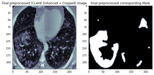
The preprocessing steps are the same as we did in Part I, including CLAHE enhancement and crop the lung regions in the CT scans.
One example of preprocessed CT scan and its corresponding infection mask are shown below.
Load and Prepare Data
We read in the CT scans data and their corresponding infection masks.
cts = []
lungs = []
infections = []
img_size = 224
for i in range(0, 20):
    read_nii(raw_data.loc[i,'lung_mask'], lungs, 'lungs')
    read_nii(raw_data.loc[i,'ct_scan'], cts, 'cts')
    read_nii(raw_data.loc[i,'infection_mask'], infections, 'infections')

print(len(cts), len(infections))
Drop Data with blank and NaN infection masks
blank_infections = []
for i in range(0, len(infections)):
  if np.unique(infections[i]).size == 1:
    blank_infections.append(i)
print("Number of complete black masks :" , len(blank_infections))

for index in sorted(blank_infections, reverse = True):
    del infections[index]
    del cts[index]
nan_list = []
for img_id in range(len(infections)):
    if np.isnan(infections[img_id].sum()):
        nan_list.append(img_id)
print(nan_list)
del infections[1476]
del cts[1476]
So far, all the preprocessing and data cleansing are done. We have 1614 cleaned CT scans with their corresponding infection masks. They are ready to use to train our infection prediction model. Let's first take a few samples from our cleaned dataset.
def plot_sample(array_list, color_map = 'jet'):
    '''
    Plots and a slice with all available annotations
    '''
    fig = plt.figure(figsize=(10,30))

    plt.subplot(1,2,1)
    plt.imshow(array_list[0].reshape(224, 224), cmap='bone')
    plt.title('Original Image')

    plt.subplot(1,2,2)
    plt.imshow(array_list[0].reshape(224, 224), cmap='bone')
    plt.imshow(array_list[1].reshape(224, 224), alpha=0.5, cmap=color_map)
    plt.title('Infection Mask')
    plt.show()

for index in [100,110,120,130,140,150]:
    plot_sample([cts[index], infections[index]])


Building Model
Instead of using Res-UNet as we used in previous posts, we will use basic UNet models this time. Because I found it easier to train on this task. I've tried Res-UNet beforehand with different hyperparameters, but it converged very slowly. By contrast, basic UNet converges faster on this task.
def build_infection_model(input_layer, start_neurons, DropoutRatio = 0.25):

    conv1 = Conv2D(start_neurons * 1, (3, 3), activation="relu", padding="same")(input_layer)
    conv1 = Conv2D(start_neurons * 1, (3, 3), activation="relu", padding="same")(conv1)
    conv1 = BatchNormalization()(conv1)
    pool1 = MaxPooling2D((2, 2))(conv1)
    pool1 = Dropout(DropoutRatio)(pool1)

    conv2 = Conv2D(start_neurons * 2, (3, 3), activation='relu', padding="same")(pool1)
    conv2 = Conv2D(start_neurons * 2, (3, 3), activation='relu', padding="same")(conv2)
    conv2 = BatchNormalization()(conv2)
    pool2 = MaxPooling2D((2, 2))(conv2)
    pool2 = Dropout(DropoutRatio)(pool2)

    conv3 = Conv2D(start_neurons * 4, (3, 3), activation="relu", padding="same")(pool2)
    conv3 = Conv2D(start_neurons * 4, (3, 3), activation="relu", padding="same")(conv3)
    conv3 = BatchNormalization()(conv3)
    pool3 = MaxPooling2D((2, 2))(conv3)
    pool3 = Dropout(DropoutRatio)(pool3)

    conv4 = Conv2D(start_neurons * 8, (3, 3), activation="relu", padding="same")(pool3)
    conv4 = Conv2D(start_neurons * 8, (3, 3), activation="relu", padding="same")(conv4)
    conv4 = BatchNormalization()(conv4)
    pool4 = MaxPooling2D((2, 2))(conv4)
    pool4 = Dropout(DropoutRatio)(pool4)

    convm = Conv2D(start_neurons * 16, (3, 3), activation="relu", padding="same")(pool4)
    convm = Conv2D(start_neurons * 16, (3, 3), activation="relu", padding="same")(convm)


    deconv4 = Conv2DTranspose(start_neurons * 8, (3, 3), strides=(2, 2), padding="same")(convm)
    uconv4 = concatenate([deconv4, conv4])
    uconv4 = BatchNormalization()(uconv4)

    uconv4 = Conv2D(start_neurons * 8, (3, 3), activation="relu", padding="same")(uconv4)
    uconv4 = Conv2D(start_neurons * 8, (3, 3), activation="relu", padding="same")(uconv4)


    deconv3 = Conv2DTranspose(start_neurons * 4, (3, 3), strides=(2, 2), padding="same")(uconv4)
    uconv3 = concatenate([deconv3, conv3])
    uconv3 = BatchNormalization()(uconv3)

    uconv3 = Conv2D(start_neurons * 4, (3, 3), activation="relu", padding="same")(uconv3)
    uconv3 = Conv2D(start_neurons * 4, (3, 3), activation="relu", padding="same")(uconv3)


    deconv2 = Conv2DTranspose(start_neurons * 2, (3, 3), strides=(2, 2), padding="same")(uconv3)
    uconv2 = concatenate([deconv2, conv2])
    uconv2 = BatchNormalization()(uconv2)

    uconv2 = Conv2D(start_neurons * 2, (3, 3), activation="relu", padding="same")(uconv2)
    uconv2 = Conv2D(start_neurons * 2, (3, 3), activation="relu", padding="same")(uconv2)


    deconv1 = Conv2DTranspose(start_neurons * 1, (3, 3), strides=(2, 2), padding="same")(uconv2)
    uconv1 = concatenate([deconv1, conv1])
    uconv1 = BatchNormalization()(uconv1)

    uconv1 = Conv2D(start_neurons * 1, (3, 3), activation="relu", padding="same")(uconv1)
    uconv1 = Conv2D(start_neurons * 1, (3, 3), activation="relu", padding="same")(uconv1)


    output_layer = Conv2D(1, (1,1), activation="sigmoid")(uconv1)

    return output_layer
Define Metrics
We first define metrics for training our model. We use the dice coefficient and dice loss. Dice coeffient is the ratio between 2 * intersection (of true mask and predicted mask) and the sum of true and predicted masks. I refered to this site.
def dice_coef(y_true, y_pred):
    smooth = 1.
    y_true_f = K.flatten(y_true)
    y_pred_f = K.flatten(y_pred)
    intersection = K.sum(y_true_f * y_pred_f)
    score = (2. * intersection + smooth) / (K.sum(y_true_f) + K.sum(y_pred_f) + smooth)
    return score

def dice_loss(y_true, y_pred):
    loss = 1 - dice_coef(y_true, y_pred)
    return loss

def bce_dice_loss(y_true, y_pred):
    loss = 0.5*binary_crossentropy(y_true, y_pred) + 0.5*dice_loss(y_true, y_pred)
    return loss
Cosine Anealing Learning Rate Scheduler
We use a learning rate scheduler to help training the model. Feel free to try different hyper-parameters to tune the model.
import math
class CosineAnnealingScheduler(Callback):
    """Cosine annealing scheduler.
    """

    def __init__(self, T_max, eta_max, eta_min=0, verbose=1):
        super(CosineAnnealingScheduler, self).__init__()
        self.T_max = T_max
        self.eta_max = eta_max
        self.eta_min = eta_min
        self.verbose = verbose

    def on_epoch_begin(self, epoch, logs=None):
        if not hasattr(self.model.optimizer, 'lr'):
            raise ValueError('Optimizer must have a "lr" attribute.')
        lr = self.eta_min + (self.eta_max - self.eta_min) * (1 + math.cos(math.pi * epoch / self.T_max)) / 2
        K.set_value(self.model.optimizer.lr, lr)
        print('\nEpoch %05d: CosineAnnealingScheduler setting learning ''rate to %s.' % (epoch + 1, lr))

    def on_epoch_end(self, epoch, logs=None):
        logs = logs or {}
        logs['lr'] = K.get_value(self.model.optimizer.lr)

cosine_annealer = CosineAnnealingScheduler(T_max=7, eta_max=0.0003, eta_min=0.00003)
Training Model
We first split the augmented dataset into training and validation sets (0.8:0.2).
We train the model for 80 epochs with a batch_size of 16. We set a ModelCheckpoint to save the model with the best val_dice_coef.
cts = np.array(cts)
infections = np.array(infections)

print(cts.shape, infections.shape)
cts = cts/255.
infections = infections/255.

x_train, x_valid, y_train, y_valid = train_test_split(cts, infections, test_size=0.2, random_state=42)
print(x_train.shape, x_valid.shape)

epochs = 80
batch_size = 32

# initialize our model
inputs = Input((img_size, img_size, 1))
output_layer = build_infection_model(inputs, 32, 0.25)
# Define callbacks to save model with best val_dice_coef
checkpointer = ModelCheckpoint(filepath = 'best_infections_224_res.h5', monitor='val_dice_coef', verbose=1, save_best_only=True, mode='max')
model = Model(inputs=[inputs], outputs=[output_layer])
model.compile(optimizer=Adam(lr = 1e-5), loss=bce_dice_loss, metrics=[dice_coef])

results = model.fit(x_train, y_train, batch_size=batch_size, epochs=epochs,
                    validation_data=(x_valid, y_valid),callbacks=[checkpointer,cosine_annealer])
After training 80 epochs, we obtain a model with a best val_dice_coef of 0.867, which is not as good as our lungs masks prediction model in Part II. It is clearly shown that predicting infection lesions are much harder than prediction lung regions.
Model Evaluation
We evaluate the model performance by looking at the training and validation dice coefficient of the training process.
As we can see, the general trends of our training and validation dice coefficient are similar. This is also true to the training and validation loss.
fig, loss_ax = plt.subplots()

acc_ax = loss_ax.twinx()

loss_ax.plot(results.history['loss'], 'y', label='train loss')
loss_ax.plot(results.history['val_loss'], 'r', label='val loss')

acc_ax.plot(results.history['dice_coef'], 'b', label='train dice coef')
acc_ax.plot(results.history['val_dice_coef'], 'g', label='val dice coef')

loss_ax.set_xlabel('epoch')
loss_ax.set_ylabel('dice loss')
acc_ax.set_ylabel('dice coefficient')

loss_ax.legend(loc='upper left')
acc_ax.legend(loc='lower left')

plt.show()

Visualize the results
We compare a few examples of true infection masks and our predicted infection masks by randomly selecting 5 images from our validation set.
As we can see from the below images, our predicted masks are very close to the true masks, though there are some small lesions not covered.
def compare_actual_and_predicted(image_no):
    temp = model.predict(x_valid[image_no].reshape(1,img_size, img_size, 1))

    fig = plt.figure(figsize=(15,15))

    plt.subplot(1,3,1)
    plt.imshow(x_valid[image_no].reshape(img_size, img_size), cmap='bone')
    plt.axis("off")
    plt.title('Original Image (CT)')

    plt.subplot(1,3,2)
    plt.imshow(y_valid[image_no].reshape(img_size,img_size), cmap='bone')
    plt.axis("off")
    plt.title('True mask')

    plt.subplot(1,3,3)
    plt.imshow(temp.reshape(img_size,img_size), cmap='bone')
    plt.axis("off")
    plt.title('Predicted mask')

    plt.show()
rand = np.random.randint(0, len(x_valid), size=5)
for i in rand:
    compare_actual_and_predicted(i)


Comments
comments powered by Disqus